高性能计算服务
>
软件专区
>
最佳实践
>
LAMMPS计算热导率与Python数据后处理实践详解
热导率是描述材料导热能力的关键物理量,在半导体、纳米材料、热管理等领域具有重要应用价值。本文详细介绍如何利用分子动力学模拟软件LAMMPS计算材料热导率,并结合Python进行数据后处理与可视化分析,为相关研究提供完整的技术实践指南。
目前,超算互联网提供预编译的LAMMPS 2Aug2023版本,支持一键购买使用。本文实验测试使用intelmpi2018编译的LAMMPS版本:
https://www.scnet.cn/ui/mall/detail/goods?id=1734740469651730433&resource=APP_SOFTWARE
您可以通过“我的商品”,在“应用软件”中找到或者搜索该版本商品,点击“命令行”,即可选择区域中心、命令行快速使用软件。
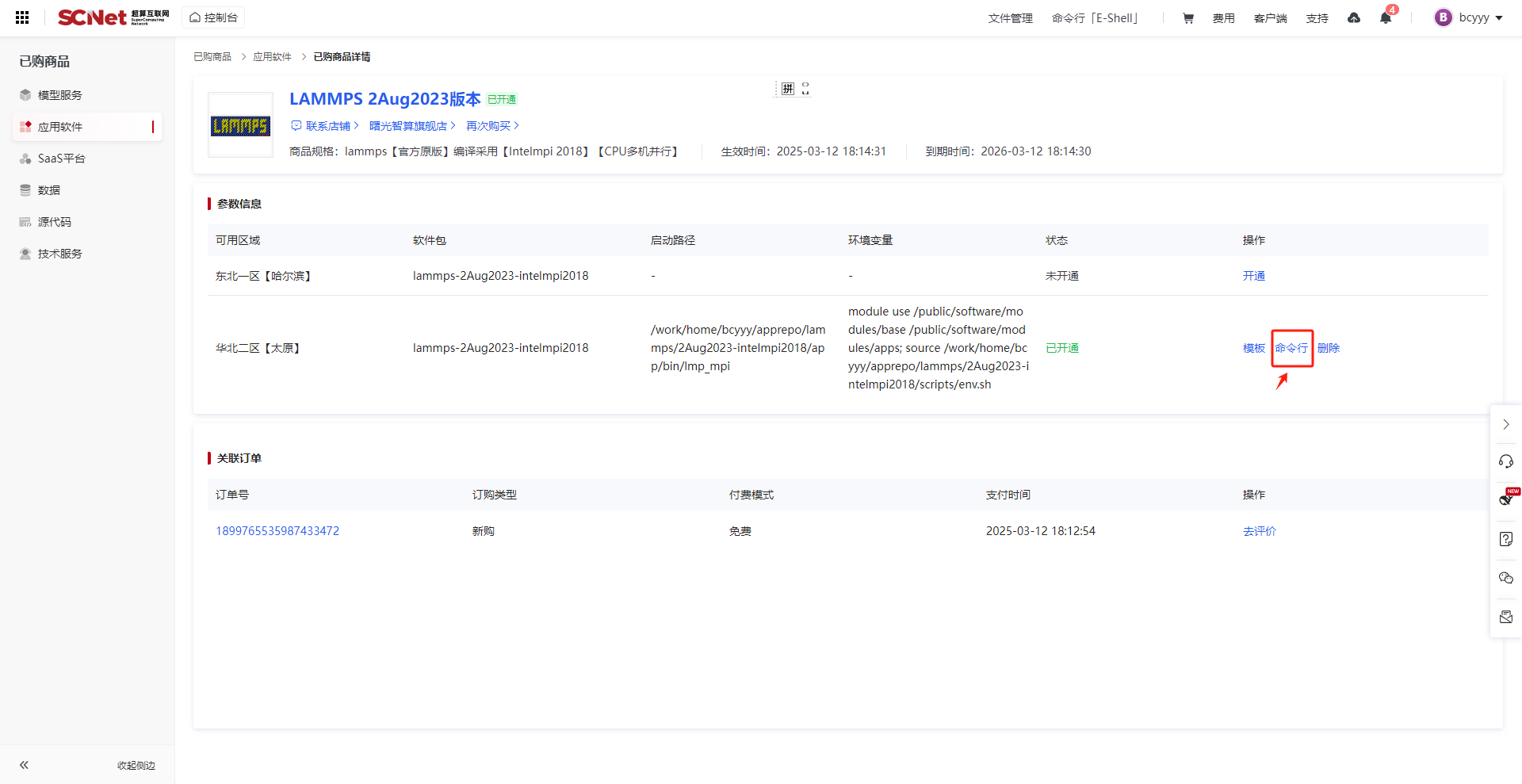
软件默认安装在家目录的apprepo下,环境变量默认放在软件scripts目录下的env.sh中,通过修改case文件夹的脚本文件得到我们的脚本文件。
#!/bin/bash
#SBATCH -J lammps #作业名称
#SBATCH -p tyhctest #队列名称
#SBATCH -N 2 #节点数量
#SBATCH --ntasks-per-node=32 #每节点核心数
module purge
source /work/home/bcyyy/apprepo/lammps/2Aug2023-intelmpi2018/scripts/env.sh

srun --mpi=pmi2 lmp_mpi -in in.*热导率计算主要基于两种方法:平衡态的格林-库博公式(Green-Kubo method)和非平衡分子动力学方法(NEMD)。本实践采用NEMD方法,通过在模拟体系两端建立温度梯度,测量稳态热流来计算热导率。根据傅里叶热传导定律,热导率κ可表示为:
κ = J/(A·∇T)
其中J为热流,A为横截面积,∇T为温度梯度。
首先需要构建合适的原子模型,本例使用硅晶体作为研究对象。硅作为半导体材料,其热导率研究具有重要的应用价值。
LAMMPS需要两个关键输入文件:控制脚本和原子结构文件。
# LAMMPS热导率计算脚本

# 基本变量设置
variable        simname index si          # 模拟名称
variable        temperature equal 300     # 系统温度(K)
variable        thigh equal 280           # 热源温度(K)
variable        tlow equal 320            # 热汇温度(K)
variable        dt equal 0.0001           # 时间步长(ps)
variable        Tdamp equal 100*${dt}     # 温度阻尼参数
variable        Pdamp equal 1000*${dt}    # 压力阻尼参数
log             log.${simname}.txt        # 日志文件

# 系统初始化
units           metal                     # 使用metal单位制
boundary        p p p                     # 周期性边界条件
timestep        ${dt}                     # 设置时间步长
atom_style      atomic                    # 原子模型类型
neigh_modify    every 1 delay 0 check yes # 邻居列表更新设置
neigh_modify    one 10000

# 读取结构数据
read_data Si.data                         # 读取硅晶体结构
mass            1 28.0855                 # 硅原子质量

# 区域与原子组定义
region          lfixed block INF INF INF INF INF 5 units box    # 左固定区域
region          rfixed block INF INF INF INF 132 INF units box  # 右固定区域
region          thigh block INF INF INF INF 5 25 units box      # 热源区域
region          tlow block INF INF INF INF 112 132 units box    # 热汇区域
group           glfixed region lfixed                           # 左固定原子组
group           grfixed region rfixed                           # 右固定原子组
group           gfixed union glfixed grfixed                    # 所有固定原子
group           gthigh region thigh                             # 热源原子组
group           gtlow region tlow                               # 热汇原子组
group           innt subtract all gfixed                        # 非固定原子组

# 势函数设置
pair_style      tersoff                                         # 选择Tersoff势
pair_coeff      * * SiC.tersoff Si                             # 载入势参数

# 计算属性定义
compute         hot_temp gthigh temp                           # 计算热源温度
compute         cold_temp gtlow temp                           # 计算热汇温度
compute         innt_temp innt temp                            # 计算非固定区域温度

# 系统能量最小化
min_style       cg                                             # 共轭梯度法
minimize        1.0e-4 1.0e-6 100 1000                         # 能量最小化参数

# 系统平衡
fix             1 all npt temp ${temperature} ${temperature} ${Tdamp} iso 1.0 1.0 ${Pdamp}
fix             555 all recenter INIT INIT INIT
thermo          100000
thermo_style    custom step temp press etotal lx ly lz
run             500000
unfix           1

# 第一次平衡运行
velocity        all create ${temperature} 28459 rot yes dist gaussian mom yes
thermo_style    custom step c_innt_temp lz ly lx pzz etotal
fix             fixed1 gfixed setforce 0.0 0.0 0.0
fix             NVE1 innt nve
fix             Temp1 innt langevin ${temperature} ${temperature} ${Tdamp} 287859 tally yes
run             500000
unfix           NVE1
unfix           Temp1

# 热导率计算
reset_timestep  0
fix             NVE3 innt nve
fix             hot1 gthigh langevin ${thigh} ${thigh} ${Tdamp} 59804 tally yes  # 热源
fix             cold1 gtlow langevin ${tlow} ${tlow} ${Tdamp} 287859 tally yes   # 热汇
run             1000000

# 温度分布采样
reset_timestep  0
compute         KE all ke/atom                                                   # 计算原子动能
variable        KB equal 8.625e-5                                                # 玻尔兹曼常数
variable        TEMP atom c_KE/1.5/${KB}                                         # 定义原子温度
compute         BLOCKS1 all chunk/atom bin/1d z lower 0.0125 units reduced       # 定义分层
fix             T_PROFILE1 all ave/chunk 10 500000 5000000 BLOCKS1 v_TEMP file temp.${simname}.txt

# 输出设置
thermo_style    custom step c_innt_temp c_hot_temp c_cold_temp f_hot1 f_cold1 etotal
fix             ave_thermo all ave/time 10000 5 100000 f_hot1 f_cold1 file thermo.${simname}.txt
run 5000000 # 运行LAMMPS data file for crystal
22950 atoms
1 atom types
0.0 40.7302 xlo xhi
0.0 40.7302 ylo yhi
0.0 150 zlo zhi
Masses
1 28.0855
Atoms #atomic
1 1 11.54023750 0.67883750 0.43741250
2 1 14.25558750 0.67883750 3.15276250
3 1 16.97093750 0.67883750 5.86811250
4 1 19.68628750 0.67883750 8.58346250
5 1 22.40163750 0.67883750 11.29881250
6 1 25.11698750 0.67883750 14.01416250
7 1 27.83233750 0.67883750 16.72951250
8 1 30.54768750 0.67883750 19.44486250
9 1 33.26303750 0.67883750 22.16021250
10 1 35.97838750 0.67883750 24.87556250
11 1 38.69373750 0.67883750 27.59091250
12 1 0.67883750 0.67883750 30.30626250
13 1 3.39418750 0.67883750 33.02161250
14 1 6.10953750 0.67883750 35.73696250
15 1 8.82488750 0.67883750 38.45231250
16 1 11.54023750 0.67883750 41.16766250
17 1 14.25558750 0.67883750 43.88301250
18 1 16.97093750 0.67883750 46.59836250
19 1 19.68628750 0.67883750 49.31371250
20 1 22.40163750 0.67883750 52.02906250
21 1 25.11698750 0.67883750 54.74441250
22 1 27.83233750 0.67883750 57.45976250
23 1 30.54768750 0.67883750 60.17511250
24 1 33.26303750 0.67883750 62.89046250
25 1 35.97838750 0.67883750 65.60581250
26 1 38.69373750 0.67883750 68.32116250
27 1 0.67883750 0.67883750 71.03651250
28 1 3.39418750 0.67883750 73.75186250
29 1 6.10953750 0.67883750 76.46721250
30 1 8.82488750 0.67883750 79.18256250
31 1 11.54023750 0.67883750 81.89791250
32 1 14.25558750 0.67883750 84.61326250
33 1 16.97093750 0.67883750 87.32861250
34 1 19.68628750 0.67883750 90.04396250
35 1 22.40163750 0.67883750 92.75931250
36 1 25.11698750 0.67883750 95.47466250
37 1 27.83233750 0.67883750 98.19001250
38 1 30.54768750 0.67883750 100.90536250
39 1 33.26303750 0.67883750 103.62071250
40 1 35.97838750 0.67883750 106.33606250
41 1 38.69373750 0.67883750 109.05141250
42 1 0.67883750 0.67883750 111.76676250
43 1 3.39418750 0.67883750 114.48211250
...
22945 1 12.89791250 37.33606250 123.98583750
22946 1 15.61326250 37.33606250 126.70118750
22947 1 18.32861250 37.33606250 129.41653750
22948 1 21.04396250 37.33606250 132.13188750
22949 1 23.75931250 37.33606250 134.84723750
22950 1 26.47466250 37.33606250 137.56258750关于输入in文件的更多设置,可以参考官方文档指导,LAMMPS官方文档: https://docs.lammps.org/
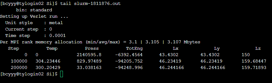
将上述输入文件保存为in文件和data文件,并放置在同目录下,通过sbatch 脚本文件来调用资源开始仿真。

tail 一下日志查看程序运行状态
热导率计算需要处理LAMMPS输出的温度分布数据和热流数据。以下是基于Python的数据分析流程:
import numpy as np
import matplotlib.pyplot as plt

# 文件路径
temp_file = "temp.si.txt"    # 温度分布数据
thermo_file = "thermo.si.txt" # 热流数据

# 读取温度分布数据
with open(temp_file, 'r') as f:
    lines = f.readlines()

# 跳过前4行标题行
data_lines = lines[4:]
temp_data = []

for line in data_lines:
    values = line.strip().split()
    # 转换为浮点数
    temp_data.append([float(val) for val in values])

temp_ave = np.array(temp_data)

# 读取热流数据
with open(thermo_file, 'r') as f:
    lines = f.readlines()

# 跳过前2行标题行
data_lines = lines[2:]
thermo_data = []

for line in data_lines:
    values = line.strip().split()
    # 转换为浮点数
    thermo_data.append([float(val) for val in values])

temperature = np.array(thermo_data)基于非平衡分子动力学方法,热导率计算公式为:κ = (Q·L)/(A·ΔT),其中Q为热流,L为系统长度,A为横截面积,ΔT为温度差。
# 参数设置
dt = 0.0001        # 时间步长(ps)
Ns = 100000        # 采样间隔
A = 4.3**2         # 横截面积(nm²)
l=14 # 长度(nm)
N_temp = len(temperature)  # 时间步数

# 筛选有效温度数据(温度大于200K)
valid_temp_data = temp_ave[temp_ave[:, 3] > 200]

# 计算温度差(选取稳定区域的代表点)
temp_difference = temp_ave[12][3] - temp_ave[61][3]
print(f"温度差: {temp_difference} K")

# 计算时间序列(转换为ns单位)
t = dt * np.arange(1, N_temp + 1) * Ns / 1000

# 计算热流(能量传递率)
# 热源热流计算
Q1 = (temperature[N_temp//2-1][1] - temperature[-1][1]) / (N_temp/2) / dt / Ns
# 热汇热流计算
Q2 = (temperature[-1][2] - temperature[N_temp//2-1][2]) / (N_temp/2) / dt / Ns
# 取平均热流(单位:eV/ps)
Q = (Q1 + Q2) / 2
print(f"平均热流: {Q} eV/ps")

# 计算热导率(单位:W/mK)
G = 160 * Q *l/ A / temp_difference  # 160是单位转换因子
print(f"热导率: {G} W/mK")可视化是理解热导率计算结果的重要手段。以下代码生成三个关键图形:温度分布曲线、热源热流变化和热汇热流变化。
# 创建多子图布局
plt.figure(figsize=(12, 10))

# 温度分布图
plt.subplot(2, 2, 1)
plt.plot(valid_temp_data[:, 1], valid_temp_data[:, 3], 'o-', color='blue')
plt.xlabel('坐标位置')
plt.ylabel('温度 (K)')
plt.title('系统温度分布')
plt.grid(True)

# 热流对比图(原始数据)
plt.subplot(2, 2, 3)
plt.plot(temperature[:, 0]*dt/1000, temperature[:, 1], 'o-', color='red', label='热源')
plt.plot(temperature[:, 0]*dt/1000, temperature[:, 2], 'o-', color='blue', label='热汇')
plt.xlabel('时间 (ns)')
plt.ylabel('热流 (eV)')
plt.title('热流时间演化')
plt.legend()
plt.grid(True)

# 热流对比图(热汇取绝对值)
plt.subplot(2, 2, 2)
plt.plot(temperature[:, 0]*dt/1000, temperature[:, 1], 'o-', color='red', label='热源')
plt.plot(temperature[:, 0]*dt/1000, -temperature[:, 2], 'o-', color='blue', label='热汇(绝对值)')
plt.xlabel('时间 (ns)')
plt.ylabel('热流 (eV)')
plt.title('热流对称性分析')
plt.legend()
plt.grid(True)

# 优化布局并保存图像
plt.tight_layout()
plt.savefig('thermal_conductivity_analysis.png', dpi=300, bbox_inches='tight')
plt.show()
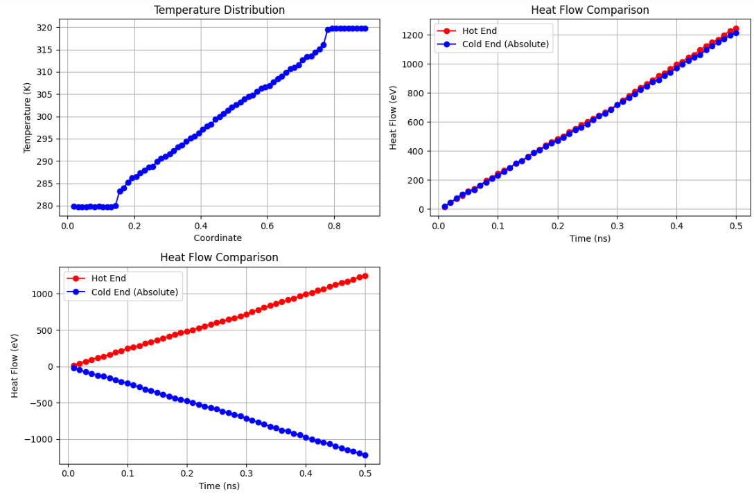
与文献中的计算结果接近
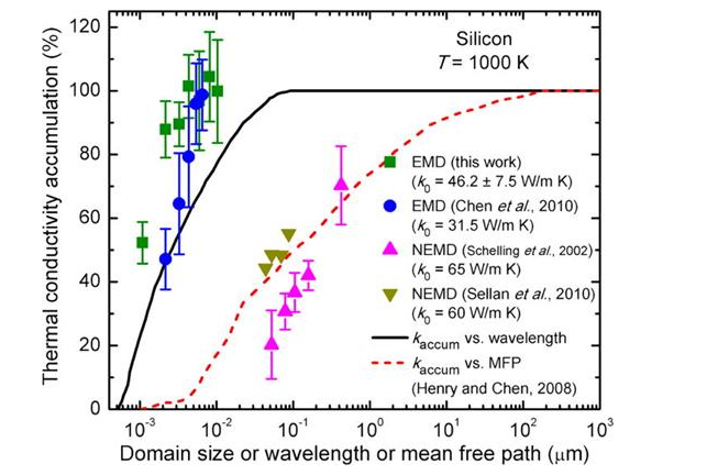
由于纳米材料有强烈的尺寸效应,大家可以进一步改变模型尺寸进行进一步研究。
本文详细介绍了使用LAMMPS计算材料热导率的完整流程,包括模拟体系的构建、LAMMPS输入文件的准备、高性能计算环境配置,以及基于Python的数据后处理与可视化分析。通过这一流程,研究人员可以准确评估各类材料的热传导性能,为新型高效热管理材料的设计提供指导。
参考资料: